
Dollar-Cost Averaging Versus Lump-Sum Investing: Which Builds More Wealth?

In a test of rolling 20-year periods since 1926, lump-sum investing outperformed dollar-cost averaging 73% of the time.

Explains the mechanics of two strategies for getting a large amount of money into the market, along with their risks and behavioral appeal
Shows historical evidence of lump-sum investing outperforming most periods
Discusses when dollar-cost averaging may be preferred and introduces momentum-based variation
In light of the recent equity market rise, the potential for increased volatility and the several equity market crashes that have occurred over the last 30 years, a growing number of investors have become wary of putting large amounts of cash to work in the market at one time. At Quent Capital, we recently took an updated look at lump-sum investing compared to dollar-cost averaging (DCA).
What Is Dollar-Cost Averaging?
Dollar-cost averaging is a strategy by which investors gradually put money to work in the market by investing a set amount at a certain frequency (typically monthly) instead of investing it all at once—commonly referred to as lump-sum investing. The idea behind dollar-cost averaging is that a given amount of money buys more shares when prices are low and fewer shares when prices are high. Burton Malkiel discussed this principle in his seminal book “A Random Walk Down Wall Street” (W.W. Norton & Co., 1975):
“Periodic investments of equal dollar amounts in common stocks can substantially reduce (but not avoid) the risks of equity investment by ensuring that the entire portfolio of stocks will not be purchased at temporarily inflated prices. The investor who makes equal dollar investments will buy fewer shares when prices are high and more shares when prices are low. The reason why an investor is able to buy more when prices are low and less when prices are high can be explained by the following equation:
Number of Shares Purchased = Dollar Amount Invested ÷ Price per Share”
We can apply this concept to buying the whole market through an index fund or to buying a select set of securities (active management). Since the same dollar amount is being invested each month, this strategy forces investors to buy more shares at lower prices and fewer shares at higher prices.
Dollar-cost averaging is thus a type of value strategy, except it works across time rather than across stocks. Markets always fluctuate to a degree, and these up-down jumps allow the strategy to achieve an average per-share cost of the market or active portfolio that is lower than the average of the market’s levels over time.
This sounds brilliant, but in this article, I explain why it is actually less desirable than investing all of one’s assets at the beginning of the investment period.
But first, let’s settle some confusion that often arises when discussing dollar-cost averaging. I am talking about when to invest a parcel of new money that comes into the investor’s possession—that is, whether to buy the intended portfolio now or dribble it into the market over time. I am not talking about dribbling money into the market over time as you earn or save it, like one does when receiving a paycheck. Everyone does that, and they should. You can’t invest money that you don’t have yet.
The Intuitive Theory Behind Lump-Sum Investing
The most important intuitive reason why lump-sum investing is better than dollar-cost averaging is that, according to basic economic theory, the expected return on the stock market is higher than the riskless (Treasury bill or bond) rate. This is because stocks must be priced to yield a positive equity risk premium (ERP) in order for investors to choose them over riskless or low-risk stocks.
The equity risk premium varies over time, but since no one knows how it will vary in the future, it’s reasonable to assume that it will be the same in December as it is when the money is received in January. Because the equity risk premium is positive, the price of the stocks to be bought 11 months in the future is more likely to be higher than lower. Dollar-cost averaging is a bet that the market will instead fall, then rise again later. This is a possible outcome, but it has a less than 50% probability. So, you should invest your new money all at once, right now. That’s the ground-level intuition.
Here’s another way to express this: You must think that stocks are going to go up, or you wouldn’t be buying them. Why do you think stocks will go down first? If you think they’re going to go down, why buy them at all?
An advocate of dollar-cost averaging would say that they’re hedging their bets. Nobody knows the future direction of the markets, so hedging is rational. But dollar-cost averaging is a strange way to put on a hedge. If you’re not sure whether stocks will go up or down, why not hedge by constantly implementing a lower-beta strategy than the market? Conventionally, that is how investors diversify: by holding different assets at the same time so that the ups of one cancel out the downs of the other.
What Is Time Diversification, and Is It Beneficial?
Some proponents of dollar-cost averaging argue that time diversification strategies like these are beneficial because they reduce risk. On average, a portfolio that is only partly invested is less risky over time than one that is fully invested all of the time. If it is desirable to diversify between stocks and cash (or another low-risk asset like bonds) at any given point in time, what’s wrong with diversifying across time, holding more cash at the beginning of the investment period and more stocks as time passes?
What’s wrong is that, unlike the benefits of diversification across assets at a given point in time, the supposed benefits of time diversification do not exist. In a 1994 Financial Analysts Journal issue, celebrated financial analyst and investment manager Mark Kritzman wrote, “It is an indisputable mathematical fact that if you prefer a riskless asset to a risky asset given a three-month horizon, you should also prefer a riskless asset to a risky asset given a 10-year horizon,” presuming your risk aversion does not change over time.
This means that your favored allocation at the beginning of the investing year given market conditions and your own risk preferences will be the same in the second month, the third month and so forth through the end of the year. Unless there is a compelling reason, the asset mix should not change over time. A strategy that is low risk at the beginning of the year and gets riskier over time until it is high risk at the end of the year makes no sense.
Historical Comparison of the Two Strategies
To compare dollar-cost averaging and lump-sum investing over longer time horizons, we ran our own simulations using a 20-year investment period as well as one-year investment periods.
We tested the two strategies over the period from January 1, 1926, through September 30, 2025. The initial portfolio was assumed to be $1 million in cash, and the only investments available were cash and the S&P 500 index. (The S&P 90 index, the S&P 500’s predecessor, was used until March 1957.) Throughout this analysis, “the S&P” means the total return, including dividends, on the index. The strategies are explained below.
Dollar-Cost Averaging Strategy: 1/12th of the initial portfolio was invested in the S&P at the beginning of each month. This means that $83,333 was invested on January 1 of a given year and an additional $83,333 was invested on the first day of each month until December 1, when the entire $1 million was invested in equities.
Lump-Sum Strategy: The entire $1 million portfolio was invested in the S&P at the beginning of the first month and held without modification for the rest of the year. In other words, the portfolio was completely invested on Day 1.
For the purposes of this study, we assumed zero transaction costs. This assumption favors the dollar-cost averaging strategy since, by design, dollar-cost averaging involves much more trading, resulting in higher transaction costs. The objectives of this backtest were twofold:
We identify which strategy was historically superior by comparing portfolio values at the end of the 12th month for all of the rolling one-year periods (rolled monthly). Thus, we computed the returns for each strategy for 1,186 rolling 12-month periods, the first running from January 1, 1926, to December 31, 1926, and the last running from October 1, 2024, to September 30, 2025.
We calculate the average difference between the dollar amounts of the two strategies for rolling 20-year investment periods. In each 20-year period, we used dollar-cost averaging only in the first 11 months, so that after the end of the first year, both strategies were fully invested in the S&P for the subsequent 19 years. There was a total of 958 20-year periods, with the first one running from January 1, 1926, to December 31, 1945, and the last one running from October 1, 2005, to September 30, 2025.
To indicate which strategy performed better historically, we assigned a value of 1 to the dollar-cost averaging strategy if it won—that is, had a larger portfolio value—by the end of the 12th month and a value of 0 if it lost. We likewise assigned a value of 1 to the lump-sum strategy if it won by the end of the 12th month and a value of 0 if it lost. Note that the performance of the two portfolios was identical after one year because both were fully invested in the S&P; they only differed in the first year. It is critical to remember this last part because we’d expect the performance difference to be much less, on an annualized basis, over a 20-year period where the two portfolios were identical for 19 of the 20 years than it is over one-year holding periods where the portfolios were profoundly different for most of the year.
This methodology was repeated for every rolling 20-year holding period, and we added up the values of 1 for each strategy.
As shown in Figure 1, the lump-sum (LS) strategy outperformed the dollar-cost averaging strategy in 696 out of the 958 periods (73% of the time). Nearly three out of four times, one would have been better off investing a lump sum than using a dollar-cost averaging strategy.

On average, at the end of a 20-year period, an investor who chose the lump-sum strategy would have had $398,770 more (per $1 million initially invested) than an investor who chose the dollar-cost averaging strategy. The average ending dollar amounts over the 12-month and 20-year rolling periods for both the lump-sum strategy and the dollar-cost averaging strategy can be seen in Figure 2. Since the strategies were fully invested by the end of the first year, both strategies have the same returns from the beginning of Year 2 through the end of Year 20. All of the outperformance is a result of the difference between the strategies during the first year. (Remember that, during this first year, the lump-sum strategy was fully invested and the dollar-cost averaging strategy was gradually invested.) On average, over each 12-month rolling period (that had a corresponding 20-year period), the lump-sum strategy outperformed the dollar-cost averaging strategy by $59,732. The $398,770 average difference at the end of the 20 years corresponds to this average difference of $59,732 obtained at the end of the first year compounded at the S&P’s rate of return.

While these differences may not seem huge, they are between 6% (the one-year case) and 40% of initial capital invested. The remarkable 20-year outcome is entirely driven by the first year’s difference, compounded at the S&P’s return for the next 19 years. (In annualized terms, the lump-sum strategy had only a 0.22% per year advantage over the dollar-cost averaging strategy because the large first-year benefit was spread over the remaining 19 years.) Thus, the initial advantage of the lump-sum strategy had a profound effect on terminal wealth, almost certainly larger than one might guess from the small annualized “alpha.”
Looking at a Representative Single Year
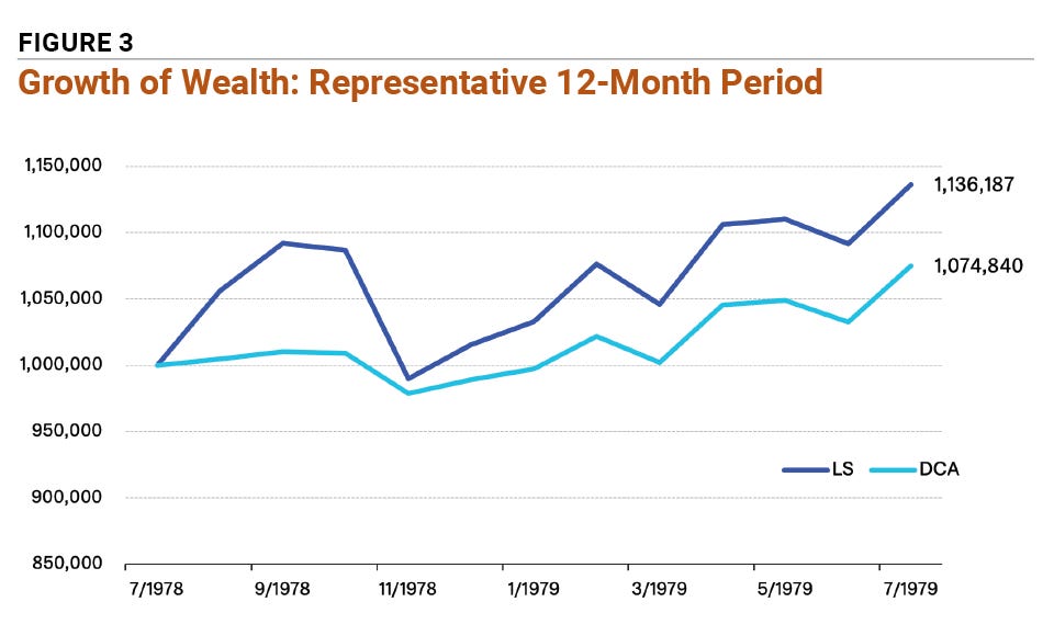
It is instructive to home in on a single representative or typical year. Figure 3 shows a one-year example: the 12-month period from July 1, 1978, through June 30, 1979, in which the lump-sum strategy outperformed the dollar-cost averaging strategy by $61,347 (per $1 million invested).
We call this a representative 12-month period because the difference in performance between the strategies in that year was similar to the average difference in performance over all the years. In other words, the performance shown in Figure 3 is more or less what can be expected from the lump-sum strategy relative to the dollar-cost averaging strategy, on average.
Analysis of Winning and Losing Periods for Dollar-Cost Averaging
Figure 4 comprises two charts showing that, in the 20-year periods when dollar-cost averaging outperformed lump-sum investing (approximately 30% of the time), the magnitude of that outperformance was less than when lump-sum investing outperformed dollar-cost averaging. Specifically, during the 696 20-year periods in which lump-sum investing did better than dollar-cost averaging, the average cumulative outperformance was $822,017 on our initial $1 million investment. During the 262 20-year periods in which dollar-cost averaging did better than lump-sum investing, the average cumulative outperformance was $725,583.


To sum up this analysis, the lower frequency of dollar-cost averaging outperformance, coupled with the lesser amount of outperformance when dollar-cost averaging outperformed, resulted in average 20-year outperformance of lump-sum investing over dollar-cost averaging of $398,770.
Conclusion
Dollar-cost averaging has been a popular investing strategy with individual investors and is still recommended by many investing professionals. Although theoretical and empirical data demonstrate that dollar-cost averaging is inferior to lump-sum and buy-and-hold strategies, it is important to understand the underlying reasons that cause investors to choose dollar-cost averaging and investing professionals to recommend it. Risk-averse investors who may be unwilling to invest into risky assets all at once find the piecemeal approach of dollar-cost averaging strategies emotionally comforting.
Quent Capital research has shown that a momentum dollar-cost averaging approach—which involves investing more or less than the basic dollar-cost averaging amount depending on whether the market went up or down, respectively, in the previous month—results in higher returns than basic dollar-cost averaging. Momentum dollar-cost averaging is grounded in the notion of piecemeal investing that investors find appealing, but involves a slight modification that improves expected return. (See the box below for more information about this approach.)
Though momentum dollar-cost averaging is by no means an optimal solution, this small deviation from the basic strategy is a significant step in reconciling rational investing principles with irrational investor behavior.